Demystifying (a light variant of) the Karush-Kuhn-Tucker conditions with full proofs for the linear program with logarithmic barrier used in Interior Point Algorithms

Daniel Porumbel

I wrote this document because I had in my mind (consciously or unconsciously) the same reasons I accidentally found at www.onmyphd.com :

1. It gives me a personal reference that I can go back and remember what I need.
2. It helps consolidate my knowledge about the topic by forcing me to explain it.
3. It gives me the satisfaction of knowing that people are learning something from me.

We take a first step towards showing how the constrained optimum of a function has to satisfy the (Karush-Kuhn-Tucker) KKT conditions. We will not prove that the presented KKT conditions are necessary in the most general sense, because we will not discuss the regularity conditions (Footnote 3). However, towards the end of this manuscript we will show the KKT conditions are necessary and sufficient for a barrier linear program used in interior point methods.  

Consider differentiable functions $f,g_1,g_2,h:\mathbb{R}^n\to\mathbb{R}$ and the program:

$$\max f(x_1,x_2,\dots x_n)$$

$$h(x_1,x_2,\dots x_n)=0$$

$$g_1(x_1,x_2,\dots x_n)\leq 0$$

$$g_2(x_1,x_2,\dots x_n)\leq 0$$

Suppose this program has a constrained maximum at point $P=<x^*_1,x^*_2,\dots x^*_n>$ such that $h(P)=0$, $g_1(P)=0$ and $g_2(P)<0$. We will show this point satisfies the KKT conditions by first addressing the constraints individually and then joining the respective conditions. In fact, we will see that the KKT conditions are verified by all local maxima of $f$ in above program.

 

1) Let us first address the equality constraint individually. Consider any (contour) curve $r(t)=<x_1(t),x_2(t),\dots x_n(t)>$ on the surface of $h(x_1,x_2,\dots x_n)=0$ with $r(0)=P=<x^*_1,x^*_2,\dots x^*_n>$ and $t\in \mathbb{R}$. This curve has to satisfy $h(r(t))=0$. Differentiating this with respect to $t$ we obtain via the chain rule (and a notation abuse discussed below):

$$0=(h(r(0)))'=\frac{\partial h}{\partial x_1} \bigg\rvert_{P}\frac... ...n}\bigg\rvert_{P} \frac{dx_n}{dt}\bigg\rvert_{0} =\nabla h\rvert_{P}\cdot r'(0)$$ (1)

We used the following notation abuse: the use of $x_i$ in a denominator $\partial x_i$ refers to the variable $x_i$, while the use of $x_i$ in a numerator $dx_i$ refers to an element of function $r(t)=<x_1(t),x_2(t),\dots x_n(t)>$.

However, the gradient of $h$ in $P$ is thus perpendicular to (the tangent of) any curve¹$r(t)$ that belongs to the surface of $h(x_1,x_2,\dots x_n)=0$. Consider now the function $f(r(t))$ and observe its derivative with respect to $t$ in 0 needs to be zero, because otherwise one could move away from $P$ in some direction along $r$ and increase the value of $f$. Using the chain rule as in (1), we obtain:

$$\nabla f\rvert_{P}\cdot r'(0)=0$$

The gradient of $f$ in $P$ is thus perpendicular to any curve $r(t)$ that belongs to the surface of $h(x_1,x_2,\dots x_n)=0$. Both $\nabla h\rvert_{P}$ and $\nabla f\rvert_{P}$ need to be perpendicular to the surface $h(x_1,x_2,\dots x_n)=0$ in $P$. In other words, there exists some $\lambda\in \mathbb{R}$ such that $\nabla f\rvert_{P}=\lambda \nabla h\rvert_{P}$.

 

2) We now address the first inequality constraint individually. Consider as above a curve $r(t)=<x_1(t),x_2(t),\dots x_n(t)>$ such that $g_1(r(t))\leq 0$ with $r(0)=P=<x^*_1,x^*_2,\dots x^*_n>$ and $t\geq 0$. We stated that we consider $g_1(r(0))=g_1(P)=0$. The intuition is that the curve starts at the constrained optimum $P$ and then it goes inside (or on the surface of) the constraint. As such, the right derivative in $t$ at point 0 satisfies: $(g_1(r(0)))'\leq 0$. Using the chain rule as in (1), we obtain:

$$\nabla g_1\rvert_{P}\cdot r'(0)\leq 0$$ (2)

The gradient $\nabla g_1\rvert_{P}$ is perpendicular to the level surface $g_1(x_1,x_2,\dots x_n)=0$ and it is the only direction for which (2) holds for any feasible curve $r(t), t\geq 0$.²

Since $r(0)=P$ is a constrained maximum, the function $f$ needs to be decreasing as we move along $t\geq 0$ from $t=0$. This means that the right derivative in 0 satisfies $(f(r(0)))'\leq 0$. Analogously to (2), we obtain:

$$\nabla f\rvert_{P}\cdot r'(0)\leq 0$$

This shows there exists some $\mu\geq 0$ such that $\nabla f\rvert_{P}=\mu \nabla g_1\rvert_{P}$, because $\nabla g_1\rvert_{P}$ is the only direction such that (2) holds for all feasible curves $r$. Observe we need to state $\mu\geq 0$ because otherwise the signs of the above inequalities would be reversed.

 

3) We now address the last inequality constraint. Since $g_2(P)<0$, the evolution of $f$ around $P$ does not depend on $g_2$. We can ignore $g_2$, as it plays no role in ensuring that $P$ is a local optimum.

 

Let us now join the arguments of 1), 2) and 3).

The point 1) shows that any objective function $f_1$ such that $\nabla f_1\rvert_{P}=\lambda \nabla h\rvert_{P}$ (with $\lambda\in \mathbb{R}$) allows $P$ to be maximum. By moving along any curve $r(t)$ on the level surface of $h$, we have $(f_1(r(0)))'=0$.

The point 2) shows that any objective function $f_2$ such that $\nabla f_2\rvert_{P}=\mu \nabla g_1\rvert_{P}$ (with $\mu\geq 0$) allows $P$ to be maximum. By moving along any curve $r(t)$ feasible with respect to $g_1(r(t))\geq 0$, we have $(f_2(r(0)))'\leq 0$: by going inside the constraint, the objective function decreases.

Consider now $f=f_1+f_2$. By moving from $P$ along any curve $r(t)$ with $t\geq 0$ that satisfies all constraints, we have $(f(r(0)))'= (f_1(r(0)))'+(f_2(r(0)))'\leq 0$, because the first term yields $(f_1(r(0)))'=0$ given that $r$ is feasible with respect to $h$ and the second term yields $(f_2(r(0)))'\leq 0$ because $r$ is feasible with respect to $g_1$.

We conclude that $P$ can be a constrained maximum for any objective function whose gradient has the form:³

$$\nabla f\rvert_{P}=\lambda \nabla h\rvert_{P} + \mu \nabla g_1\rvert_{P},$$

with $\mu\geq 0$. Using point 3), we can now write this as follows

$$\nabla f\rvert_{P}=\lambda \nabla h\rvert_{P} + \mu_1 \nabla g_1\rvert_{P}+ \mu_2 \nabla g_2\rvert_{P},$$

where $\mu_1\geq 0$ and $\mu_2=0$. Observe we can say $\mu_i g_i(P)=0$, for any $i\in\{1,2\}$: for $i=1$ we have $g_i(P)=0$ and for $i=2$, we have $\mu_i=0$.

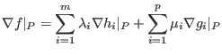
The joining argument can be generalized to more functions $h_1,h_2,\dots h_m$ and $g_1, g_2, \dots g_p$ and we obtain the KKT conditions:

• $$\nabla f\rvert_{P}=\sum_{i=1}^m\lambda_i \nabla h_i\rvert_{P} +\sum_{i=1}^p \mu_i \nabla g_i\rvert_{P}$$
• $\mu_1,\mu_2,\dots \mu_p \geq 0$
• $\mu_i g_i(P)=0,~\forall i\in[1..p]$
• $P=<x^*_1,x^*_2,\dots, x^*_n>$ is primal feasible.

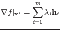
The first condition is often expressed as follows: the stationary point of the Lagrangian $f-\sum_{i=1}^m\lambda_i h_i -\sum_{i=1}^p \mu_i g_i$ in $P$ is zero. This condition can also be found by applying the Lagrangean duality and by writing the Wolfe dual problem.

Notice that if all functions are linear, it is superfluous to evaluate the gradient in $P$, because the value of the gradient is the same in all points.

(1,0)100

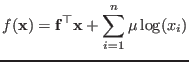
We now give a full proof of the KKT conditions for the following barrier problem used by Interior Point Methods (IPMs) for linear programming (supposing the rows $\mathbf h_i$ are linearly independent because otherwise they can be filtered).  

$$\min~ f(\mathbf x)=\mathbf f^\top \mathbf x+\sum_{i=1}^n\mu \log(x_i)$$

$$h_i(\mathbf x)=\mathbf h_i^\top \mathbf x=\bar h_i~\forall i\in [1..m]$$

There is no chance of finding an optimum solution $\mathbf x^*$ with some $x^*_i$ close to zero, because the log function exploses when its argument approaches zero. Since all involved functions are convex, this program needs to have a unique solution $\mathbf x^*$ of minimum cost. We can prove that the KKT conditions are necessary and sufficient to certify $\mathbf x^*$ is the optimal solution. The KKT conditions discussed above actually reduce to:

• $$\nabla f\rvert_{\mathbf x^*}=\sum_{i=1}^m\lambda_i \mathbf h_i$$
• $\mathbf x^*=<x^*_1,x^*_2,\dots, x^*_n>$ is primal feasible.

The necessity Take the optimal $\mathbf x^*$. The second condition is clearly necessary from the definition of $\mathbf x^*$. We prove the first condition by contradiction. Assume for the sake of contradiction that $\nabla f\rvert_{\mathbf x^*}$ can not be written as a linear combination of vectors $\mathbf h_1$, $\mathbf h_2$, $\dots$ $\mathbf h_m$. This means we can write $\nabla f\rvert_{\mathbf x^*}=\sum_{i=1}^m a_i \mathbf h_i + \mathbf z$, where $\mathbf z\neq {\bf0}$ belongs to the null space of $\mathbf h_1$, $\mathbf h_2$, $\dots$ $\mathbf h_m$, i.e., $\mathbf z^\top \mathbf h_i=0~\forall i\in[1..m]$. Let us check what happens if one moves from $\mathbf x^*$ back or forward along direction $\mathbf z$. For this, it is enough to study the function $\bar f(t)=f(\mathbf x+t\mathbf z)$. Using the chain rule, we can calculate $\bar f'(0)=\nabla f\rvert_{\mathbf x^*}^\top \mathbf z=(\sum_{i=1}^m a_i \mathbf h_i + \mathbf z)^\top = \mathbf z^\top \mathbf z>0$. By taking a sufficiently small step from $\mathbf x^*$ towards $-\mathbf z$, the function $f$ becomes smaller and the constraints $h_i$ ( $i\in[1..m])$) remain valid. This is a contradiction.

The sufficiency For the sake of contradiction, we assume there is some feasible $\mathbf x^o\neq \mathbf x^*$ such that $f(\mathbf x^*)<f(\mathbf x^o)$ that satisfies both KKT conditions, i.e, $\mathbf x^o$ is primal feasible at it can be written $\nabla f\rvert_{\mathbf x^o}=\sum_{i=1}^m\lambda_i \mathbf h_i$ for some $\lambda=[\lambda_1,~\lambda_2, \dots \lambda_m]$. Let us define the Lagrangian $\mathcal{L}(\mathbf x,\lambda)=\mathbf f(\mathbf x)-\sum_{i=1}^m \lambda_i (\mathbf h_i^\top \mathbf x-\bar h_i)$. Considering this fixed $\lambda=[\lambda_1,~\lambda_2, \dots \lambda_m]$ indicated above, this Lagrangian function is convex in the variables $\mathbf x$. Given that $\nabla f\rvert_{\mathbf x^o} - \sum_{i=1}^m\lambda_i \mathbf h_i=0$, we obtain that $\mathbf x^o$ has to be the unique stationary point of the Lagrangian function in $\mathbf x$, and so, $\mathbf x^o$ has to be the unique minimizer of the Lagrangian. This is a contradiction, because we have $\mathcal{L}(\mathbf x^*,\lambda)=f(\mathbf x^*)<f(\mathbf x^o)= \mathcal{L}(\mathbf x^o,\lambda)$.