Practical session 3: Uncertainty in classification
You can open this practical session in colab here : https://colab.research.google.com/drive/1WrzZsbsBo0xe6Zs-XAc3Rj083Ur1fzpP?usp=sharing
or download the notebook directly here.
This lab session will focus on applications based on uncertainty estimation. We will first use MC Dropout variational inference to qualitatively evaluate the most uncertain images according to the mode. Then, we’ll move to failure prediction.
Goal: Take hand on applying uncertainty estimation for failure prediction
All Imports and Useful Functions
import numpy as np
import matplotlib.pyplot as plt
from sklearn.metrics import precision_recall_curve, average_precision_score
from IPython import display
from tqdm.notebook import tqdm
from matplotlib.pyplot import imread
%matplotlib inline

import torch
import torch.nn as nn
import torch.nn.functional as F
from torch.utils.data.dataloader import DataLoader
from torchvision import datasets, transforms

use_cuda = True
device = torch.device("cuda" if use_cuda else "cpu")
kwargs = {}
#kwargs = {'num_workers': 10, 'pin_memory': True} if use_cuda else {}
#Useful plot function

def plot_predicted_images(selected_idx, images, pred, labels, uncertainties, hists, mc_samples):
    """ Plot predicted images along with mean-pred probabilities histogram, maxprob frequencies and some class histograms
    across sampliong

    Args:
    selected_ix: (array) chosen index in the uncertainties tensor
    images: (tensor) images from the test set
    pred: (tensor) class predictions by the model
    labels: (tensor) true labels of the given dataset
    uncertainties: (tensor) uncertainty estimates of the given dataset
    errors: (tensor) 0/1 vector whether the model wrongly predicted a sample
    hists : (array) number of occurences by class in each sample fo the given dataset, only with MCDropout
    mc_samples: (tensor) prediction matrix for s=100 samples, only with MCDropout

    Returns:
        None
    """
    plt.figure(figsize=(15,10))

    for i, idx in enumerate(selected_idx):
        # Plot original image
        plt.subplot(5,6,1+6*i)
        plt.axis('off')
        plt.title(f'var-ratio={uncertainties[idx]:.3f}, \n gt={labels[idx]}, pred={pred[idx]}')
        plt.imshow(images[idx], cmap='gray')

        # Plot mean probabilities
        plt.subplot(5,6,1+6*i+1)
        plt.title('Mean probs')
        plt.bar(range(10), mc_samples[idx].mean(0))
        plt.xticks(range(10))

        # Plot frequencies
        plt.subplot(5,6,1+6*i+2)
        plt.title('Maxprob frequencies')
        plt.bar(range(10), hists[idx])
        plt.xticks(range(10))

        # Plot probs frequency for specific class
        list_plotprobs = [hists[idx].argsort()[-1], hists[idx].argsort()[-2], hists[idx].argsort()[-4]]
        ymax = max([max(np.histogram(mc_samples[idx][:,c])[0]) for c in list_plotprobs])
        for j, c in enumerate(list_plotprobs):
            plt.subplot(5,6,1+6*i+(3+j))
            plt.title(f'Samples probs of class {c}')
            plt.hist(mc_samples[idx][:,c], bins=np.arange(0,1.1,0.1))
            plt.ylim(0,np.ceil(ymax/10)*10)
            plt.xticks(np.arange(0,1,0.1), rotation=60)

    plt.tight_layout()
    plt.show()
Part I: Monte-Carlo Dropout on MNIST
By appling MC Dropout variational inference method, we’re interested to obtain an uncertainty measure which can be use to spot the most uncertain images in our dataset.
# Load MNIST dataset
transform = transforms.Compose([transforms.ToTensor(), transforms.Normalize((0.1307,),(0.3081,))])
train_dataset = datasets.MNIST('data', train=True, download=True, transform=transform)
test_dataset = datasets.MNIST('data', train=False, download=True, transform=transform)

train_loader = DataLoader(train_dataset, batch_size=128, shuffle=True, **kwargs)
test_loader = DataLoader(test_dataset, batch_size=128, **kwargs)

# Visualize some images
images, labels = next(iter(train_loader))
fig, axes = plt.subplots(nrows=4, ncols=4)
for i, (image, label) in enumerate(zip(images, labels)):
    if i >= 16:
        break
    axes[i // 4][i % 4].imshow(images[i][0], cmap='gray')
    axes[i // 4][i % 4].set_title(f"{label}")
    axes[i // 4][i % 4].set_xticks([])
    axes[i // 4][i % 4].set_yticks([])
fig.set_size_inches(4, 4)
fig.tight_layout()
I.1 LeNet-5 network with dropout layers
We will use a model in the style of LeNet-5 to implement Monte-Carlo dropout variational inference.

Compared to the previous figure, the model we will implement will be defined as :
a convolutional layer with 6 channels, kernel size 5, padding 2 and ReLU activation
a max pooling layer with kernel size 2
a convolutional layer with 16 channels, kernel size 5 and ReLU activation
a max pooling layer with kernel size 2
Then flatten and:
a dropout layer with p=0.25
a fully-connected layer of size 120 and ReLU activation
a dropout layer with p=0.5
a final fully-connected layer of size 10 and ReLU activation
[CODING TASK] Implement a LeNet5-style neural network
class LeNet5(nn.Module):
    def __init__(self, n_classes=10):
        super().__init__()
        # ============ YOUR CODE HERE ============


    def forward(self, x):
        # ============ YOUR CODE HERE ============
        # Be careful, the dropout layer should be also
        # activated during test time.
        #(Hint: we may want to look out at F.dropout())

        return x
Now let’s train our model for 20 epochs using cross-entropy loss as usual.
lenet = LeNet5(n_classes=len(train_dataset.classes)).to(device)
lenet.train()
optimizer = torch.optim.SGD(lenet.parameters(), lr=0.01, momentum=0.9, weight_decay=1e-4)
criterion = nn.CrossEntropyLoss()

for i in range(20):
    total_loss, correct = 0.0, 0.0
    for images, labels in train_loader:
        images, labels = images.to(device), labels.to(device)
        optimizer.zero_grad()
        output = lenet(images)
        loss = criterion(output, labels)
        total_loss += loss
        correct += (output.argmax(-1) == labels).sum()
        loss.backward()
        optimizer.step()
    print(f"[Epoch {i + 1:2d}] loss: {total_loss/ len(train_dataset):.2E} accuracy_train: {correct / len(train_dataset):.2%}")
torch.save(lenet.state_dict(), 'lenet_final.cpkt')
# If you already train your model, you can load it instead using :
lenet.load_state_dict(torch.load('lenet_final.cpkt'))
I.2 Investigating most uncertain samples
For classification, there exists a few measures to compute uncertainty estimates: - var-ratios: collect the predicted label for each stochastic forward pass. Find the most sampled label and compute:
where \(f_x\) is the frequency of the chosen label and $T$ the number of pass.
entropy: captures the average amount of information contained in the predictive distribution.
mutual information : points that maximise the mutual informations are points on which the model is uncertain on average
[CODING TASK] Implement variational-ratio, entropy and mutual information
def predict_test_set(model, test_loader, mode='mcp', s=100, temp=5, epsilon=0.0006, verbose=True):
    """Predict on a test set given a model
    # and a chosen method to compute uncertainty estimate
    # (mcp, MC-dropout with var-ratios/entropy/mutual information
    # ConfidNet and ODIN)

    Args:
    model: (nn.Module) a trained model
    test_loader: (torch.DataLoader) a Pytorch dataloader based on a dataset
    mode: (str) chosen uncertainty estimate method (mcp, var-ratios, entropy, mi, odin)
    s: (int) number of samples in MCDropout
    temp: (int, optional) value of T for temperature scaling in ODIN
    epsilon: (float, optional) value of epsilon for inverse adversarial perturbation in ODIN
    verbose: (bool, optional) printing progress bar when predicting

    Returns:
    pred: (tensor) class predictions by the model
    labels: (tensor) true labels of the given dataset
    uncertainties: (tensor) uncertainty estimates of the given dataset
    errors: (tensor) 0/1 vector whether the model wrongly predicted a sample
    hists : (array) number of occurences by class in each sample fo the given dataset, only with MCDropout
    mc_samples: (tensor) prediction matrix for s=100 samples, only with MCDropout
    """

    model.eval()
    preds, uncertainties, labels, errors  = [], [], [], []
    mc_samples, hists = [], []

    loop = tqdm(test_loader, disable=not verbose)
    for images, targets in loop:
        images, targets = images.to(device), targets.to(device)

        if mode in ['mcp','odin']:
            model.training = False
            if mode=='odin':
                # Coding task in Section 3: implement ODIN
                images = odin_preprocessing(model,images,epsilon).to(device)
            with torch.no_grad():
                output = model(images)
            if isinstance(output,tuple):
                output = output[0]
            if mode =='odin':
                output = output / temp
            confidence, pred = F.softmax(output, dim=1).max(dim=1, keepdim=True)
            confidence = confidence.detach().to('cpu').numpy()

        elif mode in ['var-ratios', 'entropy', 'mut_inf']:
            model.training = True
            outputs = torch.zeros(images.shape[0], s, 10)
            for i in range(s):
                with torch.no_grad():
                    outputs[:,i] = model(images)
            mc_probs = F.softmax(outputs, dim=2)
            predicted_class = mc_probs.max(dim=2)[1]
            pred = mc_probs.mean(1).max(dim=1, keepdim=True)[1]
            mc_samples.extend(mc_probs)
            hist = np.array([np.histogram(predicted_class[i,:], range=(0,10))[0]
                            for i in range(predicted_class.shape[0])])
            hists.extend(hist)


            # ============ YOUR CODE HERE ============
            # hist : histogram of the predicted class for each sampling pass
            #        ie. what you need to compute the var-ratios
            # mc_probs : contains the output probability (softmax) for each MC pass.
            #            This is what you need to average over all the sampling pass
            #            to compute the entropy and the mutual information

            if mode=='var-ratios':
                # You may want to use the hist variable here
                confidence = None # <-- your implementation here>
            elif mode=='entropy':
                confidence = None # <-- your implementation here>
            elif mode=='mut_inf':
                confidence = None # <-- your implementation here>
            # =======================================

        elif mode=='confidnet':
        with torch.no_grad():
            output, confidence = model(images)
        _, pred = F.softmax(output, dim=1).max(dim=1, keepdim=True)
        confidence = confidence.detach().to('cpu').numpy()

        preds.extend(pred)
        labels.extend(targets)
        uncertainties.extend(confidence)
        errors.extend((pred.to(device)!=targets.view_as(pred)).detach().to("cpu").numpy())

    preds = np.reshape(preds, newshape=(len(preds), -1)).flatten()
    labels = np.reshape(labels, newshape=(len(labels), -1)).flatten()
    uncertainties = np.reshape(uncertainties, newshape=(len(uncertainties), -1)).flatten()
    errors = np.reshape(errors, newshape=(len(errors), -1)).flatten()

    if mode in ['var-ratios', 'entropy', 'mi']:
        hists = np.reshape(hists, newshape=(len(hists), -1))

    print(f'Test set accuracy = {(preds == labels).sum()/len(preds):.2%}')

    return preds, labels, uncertainties, errors, hists, mc_samples
Now let’s compute uncertainty estimates on the test set to visualize the most uncertainty samples
# Predicting along with var-ratios uncertainty estimates
pred_var, labels, uncertainty_var, errors_var, \
    hists, mc_samples = predict_test_set(lenet, test_loader, mode='var-ratios')
# Plotting random images with their var-ratios value
random_samples = np.random.choice(uncertainty_var.shape[0], 2, replace=False)
plot_predicted_images(random_samples, test_loader.dataset.data, pred_var, labels, uncertainty_var, hists, mc_samples)
We compare this random sample to the most uncertain images according to the var-ratio.
[CODING TASK] Visualize the top-3 most uncertain images along with their var-ratios value
# ============ YOUR CODE HERE ============
# Re-use the function 'plot_predicted_images' to visualize
# results.
top_uncertain_samples = None # <-- based on the values in uncertainty_var. You can use the .argsort() method>
plot_predicted_images(top_uncertain_samples, test_loader.dataset.data,
                    pred_var, labels, uncertainty_var, hists, mc_samples)
- [Question 1.1]: What can you say about the images themselfs. How
do the histograms along them helps to explain failure cases? Finally, how do probabilities distribution of random images compare to the previous top uncertain images?
Part II: Failure prediction
The objective is to provide confidence measures for model’s predictions that are reliable and whoseranking among samples enables to distinguish correct from incorrect predictions. Equipped with sucha confidence measure, a system could decide to stick to the prediction or, on the contrary, to handover to a human or a back-up system with,e.g.other sensors, or simply to trigger an alarm.
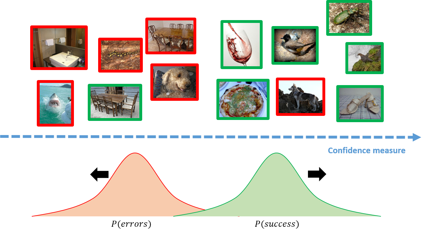
We will introduce ConfidNet, a specific method design to address failure prediction and we will compare it to MCDropout with entropy and Maximum Class Probability (MCP).
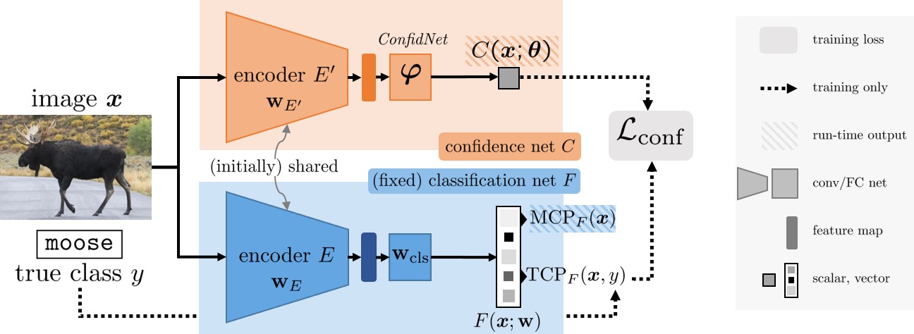
II.1 ConfidNet
By taking the largest softmax probability as confidence estimate, MCP leads to high confidence values both for correct and erroneous predictions alike. On the other hand, when the model misclassifies an example, the probability associated to the true class \(y\) is lower than the maximum one and likely to be low.
Based on this observation, we can consider instead the True Class Probability as a suitable uncertainty criterion. For any admissible input \(\pmb{x}\in \mathcal{X}\), we assume the true class \(y(\pmb{x})\) is known, which we denote \(y\) for simplicity. The TCP of a model $F$ is defined as
Theoretical guarantees. Given a properly labelled example \((\pmb{x},y)\), then:
\(\text{TCP}_F(\pmb{x},y)> 1/2\) \(\Rightarrow f(\pmb{x}) = y\), i.e. the example is correctly classified by the model;%the example has been correctly classified,
\(\text{TCP}_F(\pmb{x},y) < 1/K\) \(\Rightarrow f(\pmb{x}) \neq y\), i.e. the example is wrongly classified by the model.
However, the true classes $y$ are obviously not available when estimating confidence on test inputs. Alternatively, we can learn TCP criterion from data with an auxiliary model called ConfidNet.
ConfidNet is designed as a small multilayer perceptron composed of a succession of dense layers with a final sigmoid activation that outputs \(C(\pmb{x};\pmb{\theta})\in[0,1]\). We use a mean-square-error (MSE) loss to train this model:
class LeNet5ConfidNet(nn.Module):
    ''' A LeNet5-syle model equipped with ConfidNet auxiliary branch '''
    def __init__(self, n_classes=10):
        super().__init__()
        self.conv1 = nn.Conv2d(1, 6, 5, padding=2)
        self.maxpool1 = nn.MaxPool2d(2)
        self.conv2 = nn.Conv2d(6, 16, 5, padding=0)
        self.maxpool2 = nn.MaxPool2d(2)
        self.dropout1 = nn.Dropout(0.25)
        self.fc1 = nn.Linear(16*5*5, 120)
        self.dropout2 = nn.Dropout(0.5)
        self.fc2 = nn.Linear(120, n_classes)

        # ConfidNet Layers
        self.uncertainty1 = nn.Linear(120, 400)
        self.uncertainty2 = nn.Linear(400, 400)
        self.uncertainty3 = nn.Linear(400, 400)
        self.uncertainty4 = nn.Linear(400, 400)
        self.uncertainty5 = nn.Linear(400, 1)

    def forward(self, x):
        out = F.relu(self.conv1(x))
        out = self.maxpool1(out)
        out = F.relu(self.conv2(out))
        out = self.maxpool2(out)
        out = out.view(out.size(0), -1)
        out = self.dropout1(out)
        out = F.relu(self.fc1(out))
        out = self.dropout2(out)

        # Uncertainty prediction
        uncertainty = F.relu(self.uncertainty1(out))
        uncertainty = F.relu(self.uncertainty2(uncertainty))
        uncertainty = F.relu(self.uncertainty3(uncertainty))
        uncertainty = F.relu(self.uncertainty4(uncertainty))
        uncertainty = self.uncertainty5(uncertainty)

        pred = self.fc2(out)
        return pred, uncertainty
class SelfConfidMSELoss(nn.modules.loss._Loss):
    ''' MSE Loss for confidence learning '''
    def __init__(self, num_classes,device):
        self.nb_classes = num_classes
        self.device = device
        super().__init__()

    def forward(self, input, target):
        probs = F.softmax(input[0], dim=1)
        confidence = torch.sigmoid(input[1]).squeeze()
        labels_hot = torch.eye(10)[target.flatten()].to(device)
        loss = (confidence - (probs * labels_hot).sum(dim=1)) ** 2
        return torch.mean(loss)
We train only the ConfidNet layers for 30 epochs. During confidence learning, original classification layers are fixed to keep predictions unchanged.
lenet_confidnet = LeNet5ConfidNet(n_classes=10).to(device)
lenet_confidnet.load_state_dict(torch.load('lenet_final.cpkt'), strict=False)
lenet_confidnet.train()
optimizer = torch.optim.Adam(lenet_confidnet.parameters(), lr=1e-4)
criterion = SelfConfidMSELoss(10,device)

# Freezing every layer except uncertainty for confidence training
for param in lenet_confidnet.named_parameters():
    if "uncertainty" in param[0]:
        continue
    param[1].requires_grad = False

for i in range(30):
    lenet_confidnet.train()
    # Fine-tuning without stochasticity
    if i>20:
        # Keeping original batch norm values
        for layer in lenet_confidnet.named_modules():
            if isinstance(layer[1], torch.nn.BatchNorm2d):
                layer[1].momentum = 0
                layer[1].eval()
        # Disabling dropout
        for layer in lenet_confidnet.named_modules():
            if "dropout" in layer[0]:
                layer[1].eval()

    total_loss, correct, best_aupr = 0.0, 0.0, 0.0
    errors, uncertainty = [], []
    for images, labels in train_loader:
        images, labels = images.to(device), labels.to(device)
        optimizer.zero_grad()
        output = lenet_confidnet(images)
        probs = F.softmax(output[0], dim=1)
        pred = probs.max(dim=1)[1]
        loss = criterion(output, labels)
        loss.backward()
        optimizer.step()
        total_loss += loss
        correct += (pred == labels).sum()
        errors.extend((pred != labels.view_as(pred)).detach().to("cpu").numpy())
        uncertainty.extend(output[1].squeeze().detach().to("cpu").numpy())

    errors = np.reshape(errors, newshape=(len(errors), -1)).flatten()
    uncertainty = np.reshape(uncertainty, newshape=(len(uncertainty), -1)).flatten()
    aupr = average_precision_score(errors, -uncertainty)
    print(f"[Epoch {i + 1}] loss: {total_loss/ len(train_dataset):.2E}"+
        f"\t accuracy_train: {correct / len(train_dataset):.2%}"+
        f"\t aupr_train: {aupr:.2%}")
    if aupr>best_aupr:
    best_aupr = aupr
    torch.save(lenet_confidnet.state_dict(), 'lenet_confidnet_best.cpkt')
# If you already train your model, you can load it instead using :
# lenet_confidnet.load_state_dict(torch.load('lenet_confidnet_best.cpkt'))
II.2 Evaluate failure prediction performances
We compare the capacity of ConfidNet to detect failures with previous baselines (MCP and MCDropout with entropy).
To measure performances, we use the Area under the Precision-Recall curve (AUPR). The precision-recall (PR) curve is the graph of the precision \(= \mathrm{TP}/(\mathrm{TP} + \mathrm{FP})\) as a function of the recall \(= \mathrm{TP}/(\mathrm{TP} + \mathrm{FN})\) where \(\mathrm{TP}\), \(\mathrm{TN}\), \(\mathrm{FP}\) and \(\mathrm{FN}\) are the numbers of true positives, true negatives, false positives and false negatives respectively. In our experiments, classification errors are used as the positive detection class.
[CODING TASK] Compute precision and recall vectors along with AUPR score for ConfidNet
# ============ YOUR CODE HERE ============
# We use predict_test_set function to obtain confidence estimates
# with previous model, choosing 'confidnet' mode.
# Then calculate the precision, recall and aupr
# with sklearn functions.
# /!\ In failure prediction, errors are consider
# as the positive class

_, _, uncertainty_confidnet, errors_confidnet, _, _ = predict_test_set(lenet_confidnet, test_loader, mode='confidnet')

aupr_confidnet = # <-- use average_precision_score()
precision_confidnet, recall_confidnet, _ = # <-- use precision_recall_curve()
[CODING TASK] Same with MCP
# ============ YOUR CODE HERE ============
# Mode = 'mcp'

_, _, uncertainty_mcp, errors_mcp, _, _ = predict_test_set(lenet, test_loader, mode='mcp')
aupr_mcp = # <-- use average_precision_score()
precision_mcp, recall_mcp, _ = # <-- use precision_recall_curve()
[CODING TASK] Same with MCDropout
# ============ YOUR CODE HERE ============
# Mode = 'entropy'

_, _, uncertainty_ent, errors_ent, _, _ = predict_test_set(lenet, test_loader, mode='entropy')
aupr_ent = # <-- use average_precision_score()
precision_ent, recall_ent, _ = # <-- use precision_recall_curve()
Let’s look at the comparative results for failure prediction
plt.figure(figsize=(7,7))
plt.plot(recall_mcp, precision_mcp, label = f'MCP, AUPR = {aupr_mcp:.2%}')
plt.plot(recall_ent, precision_ent, label = f'MCDropout (Entropy), AUPR = {aupr_ent:.2%}')
plt.plot(recall_confidnet, precision_confidnet, label = f'ConfidNet, AUPR = {aupr_confidnet:.2%}')
plt.title('Precision-recall curves for failure prediction')
plt.xlabel('Recall')
plt.ylabel('Precision')
plt.legend()
plt.show()
[Question 2.1]: Compare the precision-recall curves of each method along with their AUPR values. Why did we use AUPR metric instead of standard AUROC?