Codes
Exercice 1 : K-Means
On va appliquer l’algorithme des K-Means sur la base MNIST, et interpréter le résultat de l’algorithme. On va commencer par récupérer les données:
from keras.datasets import mnist
import matplotlib.pyplot as plt
import numpy as np
from sklearn import cluster
import scipy.stats as st

# the data, shuffled and split between train and test sets
(X_train, y_train), (X_test, y_test) = mnist.load_data()
X_train = X_train.reshape(60000, 784)
X_test = X_test.reshape(10000, 784)
X_train = X_train.astype('float32')
X_test = X_test.astype('float32')
X_train /= 255
X_test /= 255
print(X_train.shape[0], 'train samples')
print(X_test.shape[0], 'test samples')
On utilise la classe KMeans du module cluster pour calculer le résultat du K-Means, en utilisant la méthode fit sur les données de test (10000 images) :
from sklearn import cluster
kmeans = cluster.KMeans(n_clusters=10, init='random').fit(X_test)
print("******** KMEANS completed ********")
On va ensuite analyser le résultat de chaque cluster, en analysant la répartition des classes (catégories des digits de 0 à 9) :
class_hists = np.zeros((10,10))
entropies = np.zeros(10)
for i in range(10):
 y_predi = y_test[kmeans.labels_==i]
 class_hists[i,:] = np.histogram(y_predi, range=(0,9))[0]
 entropies[i] = st.entropy(class_hists[i,:])

print("Matrix of cluster vs class distribution \n", class_hists)
print("entropies=", entropies)
On peut ensuite afficher le cluster dont la répartition des classes est la moins et la plus homogène :
indmin = np.argmin(entropies)
indmax = np.argmax(entropies)

print("Cluster ", indmin," with minimum entropy =",entropies[indmin])
imc = X_test[kmeans.labels_==indmin]
plt.figure(figsize=(7.195, 3.841), dpi=300)
for i in range(200):
 plt.subplot(10,20,i+1)
 plt.imshow(imc[i,:].reshape([28,28]), cmap='gray')
 plt.axis('off')

print("Cluster ", indmax," with maximum entropy =",entropies[indmax])
imc = X_test[kmeans.labels_==indmax]
plt.figure(figsize=(7.195, 3.841), dpi=300)
for i in range(200):
 plt.subplot(10,20,i+1)
 plt.imshow(imc[i,:].reshape([28,28]), cmap='gray')
 plt.axis('off')
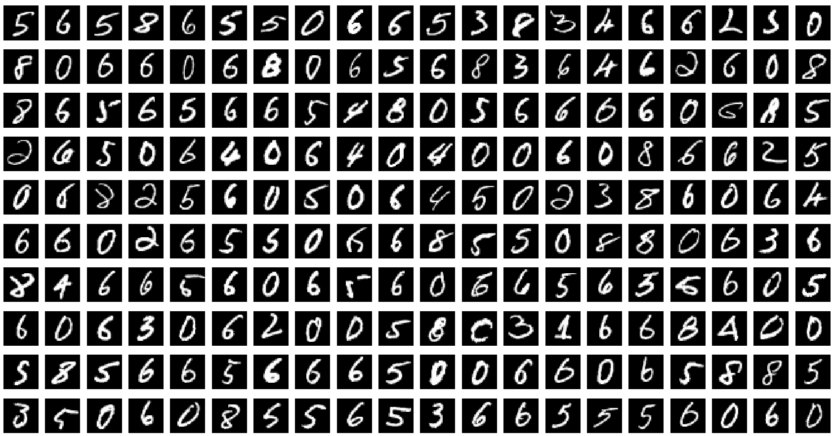
Voici un exemple de résultat, pour le cluster le plus homogène :

Et le moins homogène :
On va maintenant s’intéresser à calculer le taux de classification obtenu par l’algorithme d’apprentissage non-supervisé, si on associe un cluster à une classe :
# mapping cluster -> class
class_cluster = np.zeros(10)
accuracies = np.zeros(10) # accuracy of each cluster
indentropy = np.argsort(entropies) # we rank clusters according to entropy

class_cluster[:]=-1
class_cluster[indentropy[0]] = int(np.argmax(class_hists[indentropy[0],:])) # 1st cluster: class with min entropy
# Look in the class_histsmatrix at the cluster and class index positions
accuracies[indentropy[0]] = class_hists[int(indentropy[0]),int(class_cluster[indentropy[0]])] / np.sum(class_hists[indentropy[0],:])

for i in range(1,10):
 # New cluster index indsorted is the ist cluster in the sorted entropy list
 # We sosrt the class by increasing order of the class occurence
 indsorted = np.argsort(class_hists[int(indentropy[i]),:])
 # If the resulting class has already been attributed, we look for the next candidate
 cpt = 9
 while(list(np.where(class_cluster==indsorted[cpt])[0]) != []):
  cpt = cpt-1

 class_cluster[indentropy[i]] = int(indsorted[cpt])
 accuracies[indentropy[i]] = class_hists[int(indentropy[i]),int(class_cluster[indentropy[i]])] / np.sum(class_hists[int(indentropy[i]),:])


print("accuracies: \n", accuracies)
print("class_cluster: \n", class_cluster)

ypred = class_cluster[kmeans.labels_]
acc = np.where( ypred != y_test , 0.,1.).mean()*100.0
print("acc: \n", acc)
Exercice 2 : Algorithme de classification au plus proche voisin
On va maintenant mettre en place un algorithme de classification au plus proche voisin, qui assigne pour un exemple de test la classe de l’élément d’apprentissage le plus proche. L’enjeu va donc être de calculer une matrice de distance \(\mathbf{D}\) entre l’ensemble des exemples d’apprentissage et de test, de taille \(N_t \times N_a\), où \(N_t\) (resp. \(N_a\)) est le nombre d’exemples de test (resp. d’apprentissage). Comme :
On va calculer la norme des vecteurs d’apprentissage et de test, la matrice de produit scalaire. Ceci va permettre de calculer la matrice de distance, et de récupérer l’indice du point d’apprentissage le plus proche de chaque exemple de test, et de lui associer le label correspondant :
from keras.datasets import mnist
import numpy as np

(X_train, y_train), (X_test, y_test) = mnist.load_data()

X_train = X_train.reshape(60000, 784)
X_test = X_test.reshape(10000, 784)
X_train = X_train.astype('float32')
X_test = X_test.astype('float32')
X_train /= 255
X_test /= 255

# Dot product matrix (size 10000x60000)
PS = X_test.dot(X_train.T)

# Train norm matrix (size 10000x60000 - all rows are the same)
norm_train = np.sum(X_train**2,1)
norm_train =norm_train.reshape(60000, 1)
norm_trainr = norm_train.repeat(10000, axis=1).T

# Test norm matrix (size 10000x60000 - all colums are the same)
norm_test = np.sum(X_test**2,1)
norm_test =norm_test.reshape(10000, 1)
norm_testr = norm_test.repeat(60000, axis=1)

matdist = norm_trainr+norm_testr-2*PS
a = matdist.argmin(1)
ypred = y_train[a]

acc = np.where( ypred != y_test , 0.,1.).mean()*100.0
print("acc=",acc,"%")
Exercice 3 : Réseaux de neurones profonds
On va mettre en place un perception (réseau de neurones complètement connecté à une couche cachée) avec Keras :
from keras.models import Sequential
from keras.layers import Dense, Activation
from keras.optimizers import SGD
from keras.datasets import mnist
from keras.utils import np_utils

learning_rate = 0.5
nb_classes = 10
batch_size = 100
nb_epoch = 50

(X_train, y_train), (X_test, y_test) = mnist.load_data()

X_train = X_train.reshape(60000, 784)
X_test = X_test.reshape(10000, 784)
X_train = X_train.astype('float32')
X_test = X_test.astype('float32')
X_train /= 255
X_test /= 255

# convert class vectors to binary class matrices
Y_train = np_utils.to_categorical(y_train, nb_classes)
Y_test = np_utils.to_categorical(y_test, nb_classes)

# Building neural network
model = Sequential()
model.add(Dense(100,  input_dim=784, name='fc1'))
model.add(Activation('sigmoid'))
model.add(Dense(10,  name='fc2'))
model.add(Activation('softmax'))

model.summary()

# Training neural network
sgd = SGD(learning_rate)
model.compile(loss='categorical_crossentropy',optimizer=sgd,metrics=['accuracy'])

model.fit(X_train, Y_train,batch_size=batch_size, epochs=nb_epoch,verbose=1)

# Evaluating neural network performances
scores = model.evaluate(X_test, Y_test, verbose=0)
print("%s: %.2f%%" % (model.metrics_names[0], scores[0]*100))
print("%s: %.2f%%" % (model.metrics_names[1], scores[1]*100))
Et enfin un réseau de neurones convolutif :
from keras.datasets import mnist
from keras.models import Sequential
from keras.layers import Dense, Flatten
from keras.layers import Conv2D, MaxPooling2D
from keras.optimizers import SGD
from keras.utils import np_utils

learning_rate = 0.5
batch_size = 100
nb_classes = 10
nb_epoch = 30

(x_train, y_train), (x_test, y_test) = mnist.load_data()
x_train = x_train.reshape(x_train.shape[0], 28, 28, 1)
x_test = x_test.reshape(x_test.shape[0], 28, 28, 1)
x_train = x_train.astype('float32')
x_test = x_test.astype('float32')
x_train /= 255
x_test /= 255

# convert class vectors to binary class matrices
Y_train = np_utils.to_categorical(y_train, nb_classes)
Y_test = np_utils.to_categorical(y_test, nb_classes)

# Building neural network
s= (5,5)
input_shape = (28, 28, 1)
model = Sequential()
model.add(Conv2D(16, kernel_size=(5, 5),  activation='relu',input_shape=input_shape, padding='valid' ))
model.add(MaxPooling2D(pool_size=(2, 2)))
model.add(Conv2D(32, (5, 5), activation='relu', padding='valid'))
model.add(MaxPooling2D(pool_size=(2, 2)))
model.add(Flatten())
model.add(Dense(100, activation='sigmoid'))
model.add(Dense(nb_classes, activation='softmax'))

model.summary()

# Training neural network
sgd = SGD(learning_rate)
model.compile(loss='categorical_crossentropy',optimizer=sgd,metrics=['accuracy'])

model.fit(x_train, Y_train,batch_size=batch_size, epochs=nb_epoch,verbose=1)

# Evaluating neural network performances
scores = model.evaluate(x_test, Y_test, verbose=0)
print("%s: %.2f%%" % (model.metrics_names[0], scores[0]*100))
print("%s: %.2f%%" % (model.metrics_names[1], scores[1]*100))